Graph Neural Networks Explained: Architectures, Applications, and Research Trends in 2025–2026

Most deep learning happens on data that sits neatly in rows and columns.

Images are grids of pixels. Text is sequences of tokens. Tabular data is structured by definition. CNNs, RNNs, and Transformers were all built to handle these regular, Euclidean data structures — and they do it extremely well.

But a massive amount of real-world data doesn’t look like that at all.

Social networks are graphs. Molecular structures are graphs. Road networks are graphs. Knowledge bases are graphs. Financial transaction systems are graphs. Protein interaction networks are graphs. The internet itself is a graph.

These are relational structures — collections of entities connected by relationships — and they carry information that simply doesn’t exist in the individual entities alone. The structure is the signal.

For decades, machine learning struggled to handle this kind of data effectively.

Graph Neural Networks changed that.

In 2025–2026, GNNs have moved from academic research curiosity to production-grade technology powering fraud detection systems at major banks, drug discovery pipelines at pharmaceutical companies, recommendation engines at tech platforms, and traffic prediction systems in autonomous vehicles.

This is what the field looks like right now — and where it’s heading.

---

What Are Graph Neural Networks?

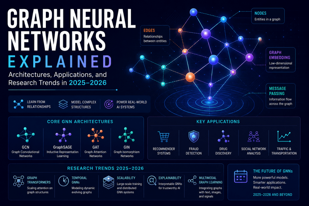
A Graph Neural Network is a class of deep learning model designed to operate directly on graph-structured data.

A graph consists of:

• Nodes (also called vertices) — representing entities
• Edges — representing relationships or connections between entities
• Node features — attribute vectors attached to each node
• Edge features — optional attribute vectors attached to each edge

Graph G = (V, E)
V = set of nodes
E = set of edges connecting nodes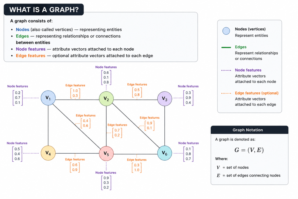

The GNN aim is to learn a representation (embedding) for each node — or for entire graphs — that captures both the node’s own features and the structural context of its position in the graph.
What makes this powerful is that the learned representation reflects not just what a node is, but who it’s connected to and how.

In social media network, a person is characterized not by their own attributes but by their relationships. A molecule’s properties depend not just on its atoms but on how those atoms are bonded. A transaction in a financial network looks different depending on the broader pattern of transactions it’s embedded in.

GNNs capture all of that.

---

Why Graphs? The Data Structure That Changes Everything

Before getting into how GNNs work, it’s worth understanding why graphs matter as a data structure.

Standard neural network architectures make an implicit assumption: that data points are independent of each other. A convolutional network processes each image independently. A language model processes each sentence (mostly) independently. The data is treated as a collection of items, not a web of relationships.

Graphs break that assumption — and that’s exactly their power.

In a graph, the relationships between data points are first class citizens. They’re not something you think of afterwards, or an implicit correlation. They’re explicitly encoded in the structure of the data itself.

This means the Graph Neural Network is able to deal with:

• Variable-size inputs — graphs can have any number of nodes and edges
• Permutation invariance — the result shouldn’t change if you reorder the nodes
• Structural information — the connectivity pattern carries information beyond node features
• Relational reasoning — understanding entities in the context of their relationships

These properties make GNNs the natural choice for a wide range of real-world problems that other architectures simply can’t handle well.

---

How GNNs Actually Work — Message Passing

The core mechanism behind most GNN architectures is called message passing — and once you understand it, the rest falls into place.

Here’s the intuition:

Each node in the graph iteratively updates its representation by aggregating information from neighboring nodes.

In a GNN, in each layer, every node:

1. Collects messages from all its neighbors — each neighbor sends some function of its current representation
2. Aggregates those messages — typically by summing, averaging, or taking the maximum
3. Updates its own representation — combining the aggregated messages with its current state through a learned function

Step 1: Message $m_{v \rightarrow u} = \text{MSG}\left(\mathbf{h}_v\right)$ for each neighbor v of u

Step 2: Aggregate $M_u = \text{AGG}\left(\left\{m_{v \rightarrow u} : v \in \mathcal{N}(u)\right\}\right)$ aggregate all neighbor messages

Step 3: Update $\mathbf{h}_u’ = \text{UPDATE}\left(\mathbf{h}_u,\, M_u\right)$ combine with own representation

After multiple layers of this process, each node’s representation captures information from its multi-hop neighborhood. After two layers, it knows about its neighbors’ neighbors. After three layers, it reaches three hops out.

This is the graph analog of a convolutional layer’s receptive field — except instead of a fixed spatial window, the “receptive field” is defined by the graph structure itself.

Different GNN architectures differ primarily in how they implement the message, aggregation, and update functions. That’s where GCN, GAT, GraphSAGE, and Graph Transformers diverge — and why each one has different strengths.

---

Core GNN Architectures

GCN — Graph Convolutional Networks

Kipf & Welling, ICLR 2017 — the architecture that started everything

Graph Convolutional Networks introduced the idea of applying convolution-like operations directly to graphs using a spectral approach — and made GNNs practical on large real-world graphs for the first time.

The core GCN layer performs a simple but powerful operation: it aggregates each node’s features with its neighbors’ features, weighted by a normalization factor derived from the degree of each node.

The propagation rule is:

à = A + I    (adjacency matrix with self-loops added)
D̃ = degree matrix of Ã
H  = node feature matrix
W  = learnable weight matrix
σ  = activation function (typically ReLU)

In plain English: each node’s new representation is a weighted average of its own features and its neighbors’ features, passed through a learnable linear transformation and a non-linearity.

The normalization by degree (the D̃ terms) prevents nodes with many neighbors from dominating the aggregation.

Why GCN matters:

GCN made graph learning practical. Before it, graph-based neural networks were too computationally expensive for large graphs. GCN’s efficient layer-wise propagation rule scaled to social networks and biological networks with millions of nodes.

Where GCN struggles:

GCN uses a fixed, symmetric aggregation — every neighbor contributes equally regardless of relevance. This works well for homophilic graphs (where connected nodes tend to be similar), but poorly for heterophilic graphs where dissimilar nodes are connected.

It also operates in a transductive setting — it can only make predictions for nodes it saw during training. New nodes require retraining.

Strengths: Efficient, well-understood, strong on homophilic graphs
Weaknesses: Fixed aggregation, transductive only, struggles with heterophily
Best for: Citation networks, social networks, biological graphs with similar connected nodes

---

GAT — Graph Attention Networks

Veličković et al., ICLR 2018 — attention comes to graphs

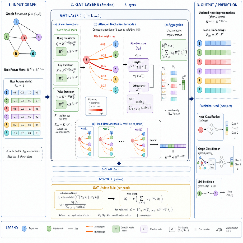
Graph Attention Networks addressed the most obvious limitation of GCN: the fact that all neighbors are treated equally.

In reality, not all neighbors are equally relevant. In a social network, some friendships are more informative than others. In a molecular graph, some atomic bonds matter more for a property than others. In a knowledge graph, some relationships carry more signal for a particular query than others.

GAT introduces learned attention weights — allowing the model to selectively focus on the most relevant neighbors for each node, rather than aggregating uniformly.

For each node u and neighbor v, GAT computes an attention coefficient:

a  = learnable attention vector
W  = learnable weight matrix
|| = concatenation

The attention coefficients α(u,v) are normalized across all neighbors using softmax, so they sum to 1. High attention = that neighbor contributes more to the update.

GAT also introduced multi-head attention — running multiple independent attention mechanisms in parallel and concatenating (or averaging) their outputs. This stabilizes training and captures different types of relationships simultaneously.

Why GAT matters:

The attention mechanism makes GAT much more flexible than GCN. It can handle graphs where different relationships have different importance, and the learned attention weights are interpretable — you can visualize which connections the model is focusing on.

Where GAT struggles:

Computing attention for every edge is expensive. On large, dense graphs, GAT’s quadratic attention complexity becomes a bottleneck. GAT v2 (Brody et al., 2022) addressed some expressiveness limitations of the original, but scalability remains a challenge.

Strengths: Learned attention weights, interpretable, handles heterophily better
Weaknesses: Expensive on large graphs, attention can be noisy with insufficient data
Best for: Heterogeneous graphs, knowledge graphs, molecular property prediction

---

GraphSAGE — Inductive Learning at Scale

Hamilton et al., NeurIPS 2017 — GNNs that generalize to unseen nodes

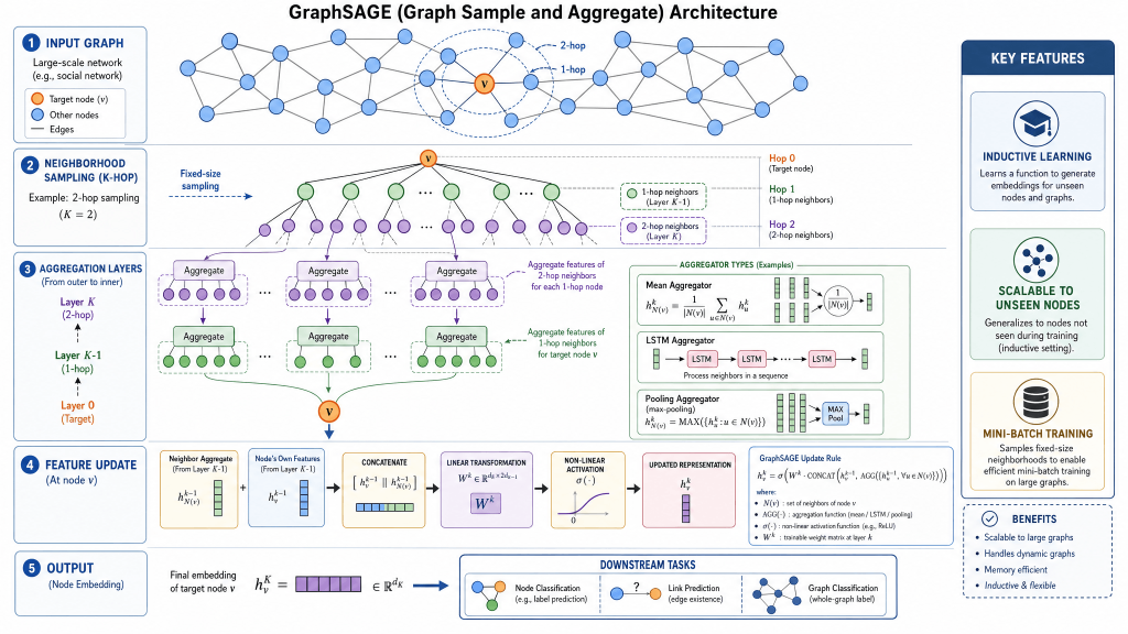
GraphSAGE (Sample and AggreGatE) solved a problem that GCN and GAT both had: neither could handle new, previously unseen nodes at inference time without retraining.

For many real-world applications — social platforms where new users join constantly, financial systems where new accounts appear, citation networks where new papers are published — this transductive limitation is a serious deployment obstacle.

GraphSAGE is inductive — it learns a function that can generate embeddings for nodes it has never seen before, by learning how to aggregate neighborhood information rather than memorizing node-specific embeddings.

The key ideas:

Neighbor sampling — instead of using all neighbors (which can be millions in large graphs), GraphSAGE samples a fixed number of neighbors at each layer. This keeps computation bounded regardless of graph size.

Learned aggregators — GraphSAGE learns an aggregation function (mean, LSTM, or max-pool) that combines sampled neighbor features.

Why GraphSAGE matters:

GraphSAGE enabled GNNs to scale to truly massive graphs. Pinterest deployed GraphSAGE on their recommendation system graph with billions of nodes and edges — one of the earliest large-scale industrial GNN deployments. It proved that GNNs could work outside academic benchmarks.

The inductive capability also means GraphSAGE generalizes across different graphs — a model trained on one graph can be applied to a different graph with the same feature space.

Strengths: Inductive learning, scales to massive graphs, generalizes to unseen nodes
Weaknesses: Sampling introduces variance, may miss important distant neighbors
Best for: Large-scale recommendation systems, dynamic graphs, industrial deployment

---

GIN — Graph Isomorphism Network

Xu et al., ICLR 2019 — the theoretically most powerful GNN

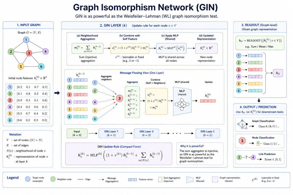
GIN took a different approach from the empirical improvements of GAT and GraphSAGE — it asked a fundamental theoretical question:

How expressive are GNNs? What graph structures can they distinguish?

Xu et al. showed that message-passing GNNs are at most as powerful as the Weisfeiler-Lehman (WL) graph isomorphism test — a classical algorithm for determining whether two graphs are structurally identical. Most GNNs (including GCN and GraphSAGE) are strictly less powerful than WL.

GIN was designed to be exactly as powerful as WL — the theoretical maximum for message-passing architectures — by using a specific aggregation function:

ε = learnable parameter (or fixed to 0)
MLP = multi-layer perceptron

The key insight is that injective aggregation — where different multisets of neighbor features always produce different outputs — is necessary and sufficient for maximum expressiveness. Simple mean or max aggregation fails this requirement for certain graph structures. Sum aggregation with an MLP passes it.

Why GIN matters:

GIN established theoretical foundations for understanding GNN expressiveness that the field still builds on. It also performs strongly in practice on graph-level tasks — predicting properties of entire graphs rather than individual nodes.

Strengths: Maximum expressiveness among message-passing GNNs, strong on graph classification
Weaknesses: Still limited by WL expressiveness ceiling, may overfit on small datasets
Best for: Graph classification, molecular property prediction, chemical fingerprinting

---

Graph Transformers — The New Frontier

2020–2026 — transformers reshape graph learning

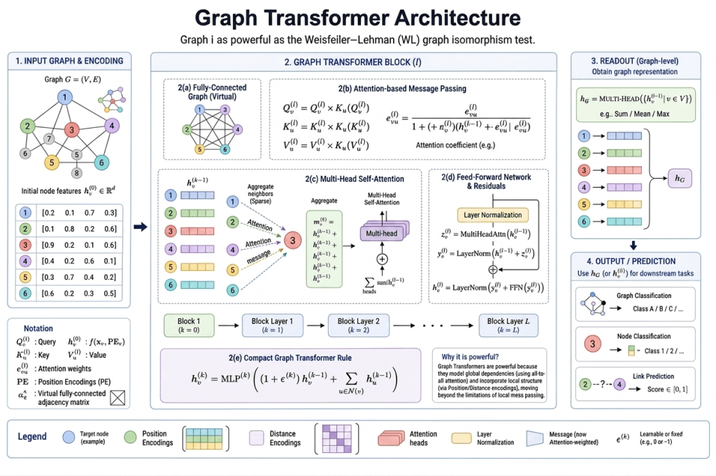
The success of Transformers in NLP and computer vision prompted a natural question: can we bring the same self-attention mechanism to graph learning?

The answer is yes — but it’s not straightforward, because graphs have properties that sequences and grids don’t.

The core challenge: Standard Transformers apply attention between all pairs of tokens (full self-attention). On a graph with N nodes, that’s O(N²) attention operations — which ignores graph structure entirely and is computationally infeasible for large graphs.

Graph Transformers solve this in different ways:

Graphormer (Ying et al., 2021) encodes graph structure into the Transformer via spatial encoding (shortest path distances between nodes) and edge encoding (features of edges on shortest paths). This lets the Transformer attend globally while still incorporating graph structure.

SAN (Kreuzer et al., 2021) uses Laplacian eigenvectors as positional encodings — providing each node with a position in the spectral geometry of the graph, giving the Transformer a sense of global structure.

GPS (Rampášek et al., 2022) — General, Powerful, Scalable Graph Transformer — combines local message passing (standard GNN layers) with global self-attention (Transformer layers) in parallel. This hybrid approach captures both local graph structure and global dependencies efficiently.

NodeFormer and SGFormer extend Graph Transformers to massive graphs with efficient approximations that avoid the full O(N²) attention computation.

Why Graph Transformers matter in 2025–2026:

Graph Transformers consistently outperform pure message-passing GNNs on benchmark tasks that require global reasoning — understanding how distant parts of a graph relate to each other. They’re particularly strong on molecular property prediction, where long-range interactions between atoms matter.

In 2025–2026, Graph Transformers are increasingly the architecture of choice for research-grade applications, while efficient variants are making their way into production systems.

Strengths: Global attention, captures long-range dependencies, strong benchmark performance
Weaknesses: Expensive without approximations, harder to scale than message-passing GNNs
Best for: Molecular property prediction, complex knowledge graph reasoning, scientific discovery

---

Architecture Comparison: 2025–2026

Architecture	Year	Aggregation	Inductive	Scalability	Best Task
GCN	2017	Normalized sum	No	Medium	Node classification
GAT	2018	Attention-weighted	No	Medium	Heterogeneous graphs
GraphSAGE	2017	Sampled aggregate	Yes	High	Large-scale production
GIN	2019	Sum + MLP	Yes	Medium	Graph classification
Graph Transformer	2021+	Global attention	Yes	Low-Medium	Molecular, scientific

---

Real-World Applications of GNNs

Financial Fraud Detection

Financial transaction networks are one of the most natural graph problems in existence.

Every transaction connects an account to a merchant. Every account connects to other accounts through shared devices, IP addresses, beneficiaries, or behavioral patterns. Fraud rarely happens in isolation — it manifests as coordinated patterns across networks of entities.

GNNs model this directly.

By representing accounts, transactions, and entities as nodes and their interactions as edges, GNNs learn to identify suspicious structural patterns — like rings of fraudulent accounts that collectively funnel money in ways no individual account reveals. GraphSAGE, GAT, and Graph Transformer variants are all actively deployed in production fraud detection systems at major financial institutions.

Recent work like MANDATE (Multi-Scale Adaptive Neighborhood Awareness Transformer) specifically addresses the challenge that fraudulent nodes often exhibit heterophily — they connect to dissimilar nodes in ways that standard GNNs struggle to model correctly.

Key architectures: GraphSAGE, GAT, Graph Transformers
Benchmark datasets: Elliptic (Bitcoin transactions), YelpChi, Amazon review fraud

---

Drug Discovery and Molecular Property Prediction

Molecules are graphs — atoms are nodes, chemical bonds are edges. This is perhaps the most natural and impactful application of GNNs.

Given a molecular graph, GNNs can predict:

• binding affinity to a target protein
• toxicity and safety profiles
• solubility and bioavailability
• molecular stability and reactivity
• ADMET properties (absorption, distribution, metabolism, excretion, toxicity)

The key advantage over fingerprint-based approaches is that GNNs learn directly from the molecular structure rather than from hand-engineered chemical descriptors. They can capture structural patterns that chemists haven’t thought to encode explicitly.

In 2025–2026, GNNs published in Nature have demonstrated near-experimental accuracy on predicting properties of crystals and novel materials — dramatically accelerating materials discovery for battery technology, catalysis, and semiconductor design.

Graph Transformers — particularly Graphormer — have shown strong performance on molecular benchmarks by capturing long-range atomic interactions that local message-passing misses.

Key architectures: GIN, Graphormer, Graph Transformers
Benchmark datasets: ZINC, MoleculeNet, OGB-molhiv, QM9

---

Recommendation Systems

Recommendation is fundamentally a graph problem: users interact with items, items belong to categories, users influence each other through social connections. This entire web of relationships is a heterogeneous graph.

Pinterest built one of the first large-scale GNN recommendation systems using GraphSAGE — deployed on a graph with billions of nodes. The GNN learns embeddings for both pins and boards simultaneously, capturing the structural relationship between them.

Subsequent systems at companies like Alibaba (GATNE), Twitter, and Uber Eats have used increasingly sophisticated GNN architectures that handle:

• temporal dynamics (how preferences change over time)
• heterogeneous node and edge types
• cold-start problems (new users or items with little interaction history)
• session-based recommendation (what to recommend next given recent behavior)

Key architectures: GraphSAGE, NGCF, LightGCN, heterogeneous GNNs
Scale: Billions of nodes and edges in production

---

Traffic and Transportation Networks

Road networks, public transit systems, and urban mobility are graphs — intersections are nodes, road segments are edges, and the features include real-time traffic conditions, historical speed patterns, weather, and events.

GNNs — specifically Spatio-Temporal Graph Neural Networks (STGNNs) — combine graph convolution (capturing spatial road network structure) with sequence modeling (capturing temporal traffic patterns) to predict:

• traffic speed and congestion 15–60 minutes ahead
• estimated travel time
• demand hotspots for ride-sharing
• optimal routing under dynamic conditions

Didi, Google Maps, and Uber all use GNN-based components in their traffic prediction and routing systems.

Key architectures: STGCN, DCRNN, Graph WaveNet, DMA-EISTGCN (2026)
Benchmark datasets: METR-LA, PEMS-BAY, PeMS traffic datasets

---

Knowledge Graph Reasoning

Knowledge graphs like Freebase, Wikidata, and domain-specific enterprise knowledge bases represent entities and their relationships. GNNs can reason over these graphs to:

• complete missing relationships (link prediction)
• answer multi-hop questions
• identify inconsistencies
• fuse knowledge from multiple sources

In 2025–2026, GNNs are being used to augment LLM reasoning — providing structured relational context that pure language model training doesn’t capture well. A GNN navigates the knowledge graph to retrieve relevant multi-hop paths, which are then passed to an LLM for natural language generation.

Key architectures: R-GCN, CompGCN, Graph Transformers
Benchmark datasets: FB15k-237, WN18RR, NELL

---

Social Network Analysis

Social platforms use GNNs for:

• community detection and clustering
• influence propagation modeling
• bot and spam account detection
• content recommendation through social graphs
• misinformation spread prediction

The graph structure of social networks — who follows whom, who interacts with whom — carries information about user behavior that individual profile features don’t capture. GNNs combine both, producing significantly better models for these tasks.

---

Research Trends in 2025–2026

1. Dynamic and Streaming Graph Neural Networks

Most GNN research assumes static graphs — fixed nodes and edges. Real-world graphs are rarely static.

Social networks evolve as friendships form and dissolve. Financial networks change with every transaction. Biological systems respond to external conditions. Road networks shift with construction and accidents.

Dynamic GNNs handle graphs where both topology and features change over time. Recent architectures incorporate instance-attention mechanisms that adapt to varying temporal frequencies — handling irregular multivariate time series on graphs that static GNNs simply cannot address.

In 2025–2026, dynamic GNNs are becoming increasingly important for:

• real-time fraud detection as transaction patterns evolve
• streaming social network analysis
• IoT sensor network monitoring
• financial market microstructure modeling

Key challenge: Efficiently updating representations as the graph changes
without recomputing everything from scratch

---

2. Scalable High-Order Feature Fusion

Standard message-passing GNNs aggregate information from immediate neighbors at each layer. To reach k-hop neighbors, you need k layers.

But stacking many GNN layers leads to over-smoothing — node representations become indistinguishable as information from distant neighborhoods blurs together. In practice, most GNNs use only 2–3 layers.

This limits their ability to capture long-range dependencies — relationships between nodes that are many hops apart but semantically connected.

2025–2026 research is addressing this through high-order feature fusion — architectures that can access multi-hop neighborhood information without the over-smoothing degradation of deep stacking. Recent work adaptively fuses features from multiple hop distances, letting the model decide which range of context is most relevant for each prediction.

This is pushing GNNs toward globally-aware representations without the computational cost of full Graph Transformer attention.

---

3. GNN and LLM Integration

This is arguably the most significant trend in GNN research in 2025–2026.

Large language models are extraordinarily powerful at processing and generating natural language. Graph Neural Networks are extraordinarily powerful at reasoning over structured relational data. Combining the two creates systems that can handle problems neither can solve alone.

The integration is happening in multiple directions:

LLMs augmented by GNNs — GNNs navigate knowledge graphs or document graphs to retrieve structured multi-hop context for LLM reasoning. Recent work uses lightweight GNNs to replace expensive LLM-based graph traversals in RAG systems, efficiently finding relevant paths at a fraction of the cost.

GNNs augmented by LLMs — LLMs provide rich semantic node features (embeddings of text descriptions) that GNNs then process over graph structure. This is particularly powerful for knowledge graphs where node and edge descriptions carry semantic meaning.

Joint architectures — unified models that process both graph structure and text simultaneously, with attention mechanisms that cross between the two modalities.

In enterprise contexts, this combination is enabling context-aware AI agents that don’t just pattern-match on text but navigate structured relationship graphs to make more informed, explainable decisions.

---

4. GNNs for Scientific Discovery

GNNs are having a genuine impact on scientific research at the frontier — not just as better tools for existing workflows, but enabling entirely new types of investigation.

Materials science: GNNs predict crystal and molecular properties with near-experimental accuracy, dramatically accelerating the search for new battery materials, catalysts, and semiconductors. Research published in Nature demonstrates this capability at scale.

Drug discovery: GNNs predict binding affinity, toxicity, and ADMET properties for novel drug candidates. The GAINET model (2025) advanced drug-drug interaction prediction. The ability to screen millions of molecular candidates computationally before any laboratory synthesis is transforming pharmaceutical R&D.

Protein structure: While AlphaFold used a different architecture, subsequent work applies GNNs to protein-protein interaction prediction, binding site identification, and protein design.

Climate modeling: Graph-based weather prediction models outperform traditional numerical weather prediction on certain tasks at dramatically lower computational cost.

The shift from “GNNs as ML tools” to “GNNs as scientific instruments” is one of the defining trends of 2025–2026.

---

5. Robustness and Certified Defenses

As GNNs move into critical infrastructure — fraud detection at banks, security monitoring at utilities, medical diagnosis systems — their robustness to adversarial attacks becomes non-negotiable.

Graph adversarial attacks are particularly subtle. An attacker can:

• add or remove a small number of edges to manipulate node classifications
• inject fake nodes into the graph with carefully crafted features
• perturb edge weights to shift model outputs

In 2025–2026, certified defense frameworks like AGNNCert and PGNNCert provide mathematically proven guarantees about model robustness — formally certifying that a GNN’s prediction won’t change under attacks below a specified magnitude. These are analogous to certified defenses in image classification but adapted for graph structure.

Training-free, model-agnostic defense frameworks are also emerging — providing robustness improvements that can be applied to existing deployed GNNs without retraining.

Why this matters: A fraud detection GNN that can be fooled by carefully crafted
transactions provides false security. Certified defenses make GNN deployment
trustworthy in regulated, high-stakes environments.

---

Challenges and Open Problems

Even with all the progress, several genuinely hard problems remain in GNN research and deployment.

Over-smoothing As GNN depth increases, node representations converge toward each other — losing the distinctive information that makes them useful for discrimination. Most production GNNs use only 2–3 layers for this reason, limiting their ability to capture long-range dependencies.

Over-squashing Information from exponentially many distant nodes gets compressed into fixed-size vectors as it passes through message-passing layers. This information bottleneck causes GNNs to lose relevant long-range signals — a fundamental architectural limitation being addressed by Graph Transformers and high-order fusion methods.

Scalability Full-graph training is infeasible for graphs with millions or billions of nodes. Sampling-based methods (GraphSAGE) and mini-batch training introduce approximation error. Finding the right balance between computational feasibility and representation quality remains an active challenge.

Heterogeneous graphs Real-world graphs often have multiple types of nodes and edges — users, items, categories, transactions, and institutions all in the same graph. Handling this heterogeneity without losing the type-specific semantics requires specialized architectures that are more complex to design and train.

Explainability When a GNN flags a transaction as fraudulent or predicts a molecule will be toxic, explaining why in human-understandable terms is hard. The distributed, relational nature of GNN representations makes attribution to specific graph structures non-trivial.

Evaluation benchmarks Many popular GNN benchmarks are too small and too simple to differentiate between architectures meaningfully. The Open Graph Benchmark (OGB) addressed this with larger, more realistic graphs — but evaluation methodology across the field remains inconsistent.

Graph-level tasks Node classification has driven most GNN research. Graph classification — predicting properties of entire graphs — is harder and less studied, despite being critical for molecular property prediction and other scientific applications.

---

Final Thoughts

Graph Neural Networks have made a journey in the last eight years that most machine learning subfields take decades to complete.

From Kipf & Welling’s GCN paper in 2017 — which made graph convolution practical for the first time — to Graph Transformers achieving near-experimental accuracy on molecular properties published in Nature, the field has moved from interesting theory to genuine scientific and industrial impact.

What’s particularly compelling about where GNNs are in 2025–2026 is the convergence happening at multiple levels simultaneously.

GNNs are converging with Transformers — bringing global attention to graph-structured data. They’re converging with LLMs — combining relational reasoning with language understanding. They’re converging with scientific computing — replacing or augmenting classical simulations in chemistry, materials science, and biology.

And they’re converging with the real world — moving from academic benchmarks to production systems at scale, with the robustness and certification requirements that real deployment demands.

The fundamental insight that makes all of this possible remains the same as it was in 2017:

The relationship between things carries information that the things themselves don’t.

Graphs encode that insight structurally. GNNs learn from it computationally. And in 2025–2026, the applications of that combination are broader and more important than anyone predicted when the field began.

---

FAQ