Kalman Filter Explained: From Classical Control Theory to Modern AI Engineering

Why Most Explanations of the Kalman Filter Get It Wrong

Here is something that bothers me about how the Kalman filter is usually taught. This article is part of the Scientias AI Labs research hub on Probabilistic Control Engineering for Generative AI.

Most textbooks introduce it as a signal processing algorithm. A way to smooth noisy sensor data. Something you use in GPS systems or aircraft navigation. Useful, sure. But the framing misses what is actually remarkable about it.

The Kalman filter is not just an engineering algorithm. It is the place where two completely separate intellectual traditions — classical control engineering and Bayesian statistical inference — discovered they had been doing the same thing all along without realizing it.

Once you see that connection, you cannot unsee it. And more importantly for anyone working in AI today, that connection turns out to be directly relevant to how modern generative AI systems work.

---

A Quick Story Before the Math

It is 1940. World War II is intensifying. Norbert Wiener, a mathematician at MIT, is working on a deeply practical problem — how do you aim an anti-aircraft gun at a moving plane when the plane’s position measurements are noisy and delayed?

The plane zigs and zags. Your radar reading is corrupted by interference. You need to predict where the plane will be in three seconds, not where it was half a second ago. And you need to do this continuously, in real time, under enormous pressure.

Wiener solved it. His solution — the Wiener filter — extracted the best possible estimate of the plane’s true position from noisy observations by combining a model of how the plane moves with a statistical model of the measurement noise.

Years later, mathematicians realized that what Wiener had built was mathematically equivalent to Bayesian estimation. A control engineer trying to track a moving target and a statistician updating a probability distribution given noisy evidence were doing identical computations. They just called them different things.

Rudolf Kalman took this insight and in 1960 published what became one of the most cited and practically influential algorithms in the history of engineering. The Kalman filter. An algorithm that is simultaneously a classical control theory tool and a Bayesian inference algorithm — and the most elegant expression of the connection between the two.

---

What the Kalman Filter Actually Does

Forget the equations for a moment. Here is the intuition.

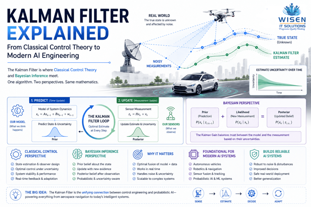
You are trying to track something — the position of a robot, the state of a physical system, the trajectory of a spacecraft. You have two sources of information. First, you have a model of how the system evolves over time. Second, you have a sensor that gives you noisy measurements of the system’s state.

Neither source is perfect. Your model makes assumptions that are never quite right. Your sensor adds noise. So what do you do?

You combine them intelligently. At each time step, the Kalman filter does two things.

First it predicts. Using your model of system dynamics, it forecasts where the system should be right now based on where it was last time step. This prediction carries uncertainty — the model is not perfect, so the prediction is not certain.

Then it updates. New sensor data arrives. The filter compares what the sensor says to what the model predicted. If they agree well, the update is small. If they disagree significantly, the update is larger. The filter weighs these two sources of information against each other based on how uncertain each one is.

The result is an estimate that is better than either the model alone or the sensor alone could provide. It is optimal in a precise mathematical sense — given Gaussian noise assumptions, no algorithm can do better.

That predict-update cycle repeats continuously. Every time step. For as long as the system runs.

---

Where Bayesian Inference Enters the Picture

If you have studied Bayesian statistics, something in that description probably sounded familiar.

The prediction step is exactly like computing a Bayesian prior — your belief about the system state before seeing new evidence, propagated forward in time using your model.

The update step is exactly like Bayesian posterior computation — combining your prior belief with new evidence to get an updated belief that is more accurate than either alone.

The Kalman gain — the number that determines how much weight to give the new sensor measurement versus the model prediction — is derived directly from the mathematics of Bayesian inference.

This is not a loose analogy. The Kalman filter under Gaussian assumptions is Bayesian inference applied to linear dynamical systems. Exactly. Mathematically. The same computation.

This equivalence is why the Kalman filter has turned out to be so foundational in modern probabilistic AI. The predict-update cycle that Rudolf Kalman formalized for aerospace navigation in 1960 is the same cycle that underlies modern state estimation in autonomous vehicles, sensor fusion systems, and increasingly, components of large AI pipelines.

---

The Math — Made Accessible

Now that you have the intuition, the equations will make more sense.

The Kalman filter maintains two quantities at each time step — a state estimate and a covariance matrix. The state estimate is your best guess of the system’s current state. The covariance matrix describes how uncertain that estimate is.

Prediction step:

Your model says that if the system was in state x at the last time step, it should be in state Ax now, where A is the state transition matrix. But your model is not perfect, so you add process noise with covariance Q.

Predicted state:

Predicted covariance:

Update step:

Your sensor gives you measurement z. The sensor observes the state through observation matrix H, with measurement noise covariance R.

You compute the Kalman gain K, which balances how much to trust the prediction versus the measurement:

Then you update:

Updated state:

Updated covariance:

That is the complete algorithm. Two steps. Repeat.

What makes it beautiful is that K automatically adapts. When R is large — meaning the sensor is noisy — K is small, and the filter trusts the model more. When P is large — meaning the model prediction is uncertain — K is large, and the filter trusts the sensor more. It finds the optimal balance automatically.

---

Python Implementation

Here is a clean Python implementation of the 1D Kalman filter — tracking position with noisy measurements:

python

import numpy as np
import matplotlib.pyplot as plt

class KalmanFilter1D:
    def __init__(self, process_variance, measurement_variance):
        self.process_variance = process_variance
        self.measurement_variance = measurement_variance
        self.estimate = 0.0
        self.estimate_error = 1.0

    def update(self, measurement):
        # Prediction step
        prediction = self.estimate
        prediction_error = self.estimate_error + self.process_variance

        # Kalman gain
        kalman_gain = prediction_error / (
            prediction_error + self.measurement_variance
        )

        # Update step
        self.estimate = prediction + kalman_gain * (
            measurement - prediction
        )
        self.estimate_error = (
            1 - kalman_gain
        ) * prediction_error

        return self.estimate

# Simulate noisy measurements
np.random.seed(42)
true_value = 10.0
measurements = true_value + np.random.normal(0, 2, 50)

# Apply Kalman filter
kf = KalmanFilter1D(
    process_variance=0.1,
    measurement_variance=4.0
)
estimates = [kf.update(m) for m in measurements]

# Plot results
plt.figure(figsize=(12, 5))
plt.plot(measurements, 'o', alpha=0.5, label='Noisy measurements')
plt.plot(estimates, linewidth=2, label='Kalman filter estimate')
plt.axhline(y=true_value, color='r', 
            linestyle='--', label='True value')
plt.legend()
plt.title('Kalman Filter: Separating Signal from Noise')
plt.xlabel('Time step')
plt.ylabel('Value')
plt.show()

Run this and watch the Kalman filter estimate converge toward the true value from noisy measurements. The filter starts uncertain and gradually becomes more confident as evidence accumulates.

---

Extended and Unscented Kalman Filters

The standard Kalman filter assumes linear dynamics and Gaussian noise. Real systems are almost never linear. This is where extensions become necessary.

The Extended Kalman Filter (EKF) handles nonlinear systems by linearizing the system dynamics around the current estimate using a first-order Taylor expansion. It is an approximation — and sometimes a rough one — but it works well for mildly nonlinear systems and has been used in countless real-world applications from robot localization to satellite tracking.

The Unscented Kalman Filter (UKF) takes a different approach. Instead of linearizing analytically, it picks a set of carefully chosen sample points — called sigma points — and propagates them through the nonlinear function exactly. It then fits a Gaussian to the resulting propagated points. For many practical systems the UKF gives significantly better performance than the EKF with comparable computational cost.

For highly non-Gaussian uncertainty, particle filters take the idea further — representing the probability distribution with a large number of random samples rather than a Gaussian approximation. They can handle arbitrary distributions but at significantly higher computational cost.

---

The Kalman Filter in Modern AI Systems

Here is where this connects directly to the work being done at the frontier of AI engineering in 2026.

Autonomous vehicles use Kalman filtering as the backbone of their sensor fusion systems. Cameras, LiDAR, radar, and GPS all provide noisy, partial information about the vehicle’s environment. The Kalman filter fuses these into coherent state estimates — tracking the positions and velocities of other vehicles, pedestrians, and obstacles with quantified uncertainty.

Generative AI control is increasingly drawing on Kalman filter principles. In Probabilistic Control Engineering — a framework that applies classical control theory concepts to generative AI systems — the predict-update cycle of the Kalman filter serves as the foundational model for how AI systems should handle uncertainty. The Kalman filter is the most direct and traceable connection between classical control engineering and modern probabilistic AI.

State space models for sequence modeling in deep learning are direct generalizations of the linear dynamical systems that the Kalman filter was designed for. Models like S4, Mamba, and other structured state space models borrow the mathematical framework directly, applying it to high-dimensional sequence data where the state is a learned latent representation rather than a physical position.

Diffusion models — the generative AI architecture behind image synthesis systems — can be understood through a Kalman filter lens. The forward diffusion process that adds noise to data and the reverse denoising process that generates clean samples from noise are structurally analogous to the prediction and update steps of a Kalman filter, generalized to handle complex non-Gaussian distributions.

The Kalman filter serves as the foundational bridge between classical control engineering and modern Probabilistic Control Engineering for Generative AI systems.

Engineers who specialize in applying these probabilistic control concepts to AI systems are increasingly known as PCE Practitioners.

---

Why Every AI Engineer Should Understand This

There is a practical reason to care about the Kalman filter beyond its direct applications.

Understanding it deeply gives you a mental model — a way of thinking about uncertainty, estimation, and the combination of prior knowledge with new evidence — that transfers directly to modern AI problems that superficially look nothing like signal processing.

When you tune a learning rate schedule, you are solving a stability problem in exactly the control-theoretic sense. When you design a reinforcement learning reward function, you are building a feedback loop. When you think about how to make a language model more reliable, you are asking a controllability question. The Kalman filter is the clearest possible illustration of these connections, because its mathematics is simple enough to understand completely while being rich enough to reveal the deep structure.

Engineers who understand the Kalman filter understand Bayesian inference more intuitively. They understand state space models more naturally. They understand why uncertainty quantification matters and how to think about it rigorously. These are exactly the skills that matter most as AI systems become more complex and the stakes of deploying them become higher.