The Three Axes of Probabilistic Control Engineering for Generative AI: Entropy Reduction, Bias Correction, and Drift Detection

Introduction — Why Generative AI Needs a Control Framework

Something bothered me for a long time about how the AI community talks about making language models more reliable. This article is part of the Scientias AI Labs research hub on Probabilistic Control Engineering for Generative AI.

The conversation is almost always about prompting, fine-tuning, or scaling. Add more data. Use a better prompt. Train longer. These are all valid techniques, but they share a common limitation — they treat the model as a black box and try to improve it from the outside. They do not provide a systematic engineering framework for understanding why the model behaves the way it does and how to control that behavior rigorously.

Control engineering solved this exact problem for physical systems sixty years ago. When Norbert Wiener was trying to control anti-aircraft guns and Rudolf Kalman was guiding spacecraft, they did not just try random adjustments until something worked. They built mathematical frameworks that described system behavior, quantified uncertainty, corrected for bias, and detected when systems drifted from desired behavior.

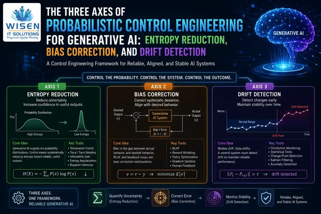
These three axes are not arbitrary. They map directly onto the three core problems of classical control engineering — uncertainty quantification, error correction, and stability monitoring. For a deeper understanding of how these classical concepts translate into modern AI engineering, see our complete guide on how Probabilistic Control Engineering borrows from Classical Control Theory.

Probabilistic Control Engineering applies that same engineering rigor to Generative AI. And when you look carefully at what Generative AI systems actually need to be controlled, three axes emerge naturally.

Axis 1 — Entropy Reduction: Generative AI outputs are probability distributions. High entropy means high uncertainty. Controlling a Generative AI system means systematically reducing entropy toward useful, reliable outputs.

Axis 2 — Bias Correction: Every control system exists to correct the gap between actual behavior and desired behavior. In Generative AI, this gap is bias — systematic deviation from correct, aligned, or useful outputs. The entire RLHF framework is a bias correction mechanism.

Axis 3 — Drift Detection: Systems change over time. Models drift. Data distributions shift. Channel conditions change. A control system that cannot detect drift cannot maintain reliable performance. Drift detection is the Kalman filter of the MLOps world.

These three axes are not arbitrary. They map directly onto the three core problems of classical control engineering — uncertainty quantification, error correction, and stability monitoring. The mathematics is the same. The engineering intuition is the same. Only the systems are different.

---

Axis 1 — Entropy Reduction

What Entropy Means in Generative AI

python

import numpy as np
import matplotlib.pyplot as plt
from scipy.stats import entropy
from scipy.special import softmax

def compute_token_entropy(logits):
    """
    Compute entropy of token probability distribution
    
    Args:
        logits: Raw model output logits (unnormalized)
    
    Returns:
        entropy_value: Shannon entropy in bits
        probabilities: Token probability distribution
    """
    # Convert logits to probabilities
    probabilities = softmax(logits)
    
    # Shannon entropy in bits
    entropy_value = entropy(probabilities, base=2)
    
    return entropy_value, probabilities

def temperature_scaling(logits, temperature):
    """
    Temperature scaling for entropy control
    
    Lower temperature = lower entropy = more confident
    Higher temperature = higher entropy = more random
    
    Args:
        logits: Raw model logits
        temperature: Scaling parameter (0 < T < inf)
    
    Returns:
        Scaled probability distribution
    """
    scaled_logits = logits / temperature
    return softmax(scaled_logits)

def nucleus_sampling(logits, p=0.9):
    """
    Nucleus (top-p) sampling for entropy reduction
    
    Keeps only the top tokens whose cumulative
    probability exceeds p, zeroing out the rest
    
    Args:
        logits: Raw model logits
        p: Nucleus probability threshold
    
    Returns:
        Filtered probability distribution
    """
    probs = softmax(logits)
    
    # Sort probabilities descending
    sorted_indices = np.argsort(probs)[::-1]
    sorted_probs = probs[sorted_indices]
    
    # Cumulative probabilities
    cumulative_probs = np.cumsum(sorted_probs)
    
    # Find nucleus cutoff
    nucleus_mask = cumulative_probs <= p
    nucleus_mask[np.sum(nucleus_mask)] = True
    
    # Zero out non-nucleus tokens
    filtered_probs = np.zeros_like(probs)
    filtered_probs[sorted_indices[nucleus_mask]] = \
        sorted_probs[nucleus_mask]
    
    # Renormalize
    filtered_probs /= filtered_probs.sum()
    
    return filtered_probs

# Simulate token distributions
np.random.seed(42)
vocab_size = 50

# High entropy scenario — model is uncertain
high_entropy_logits = np.random.randn(vocab_size) * 0.5

# Low entropy scenario — model is confident
low_entropy_logits = np.zeros(vocab_size)
low_entropy_logits[7] = 5.0  # One dominant token

# Temperature effects
temperatures = [0.3, 0.7, 1.0, 1.5, 2.0]
entropies_by_temp = []

for T in temperatures:
    scaled_probs = temperature_scaling(
        high_entropy_logits, T)
    H = entropy(scaled_probs, base=2)
    entropies_by_temp.append(H)

# Nucleus sampling effect
probs_original = softmax(high_entropy_logits)
probs_nucleus = nucleus_sampling(high_entropy_logits, p=0.9)

H_original = entropy(probs_original, base=2)
H_nucleus = entropy(probs_nucleus, base=2)

# Visualization
fig, axes = plt.subplots(1, 3, figsize=(16, 5))

# Temperature vs entropy
axes[0].plot(temperatures, entropies_by_temp,
             'o-', linewidth=2, color='steelblue')
axes[0].set_xlabel('Temperature')
axes[0].set_ylabel('Entropy (bits)')
axes[0].set_title('Temperature vs Token Entropy')
axes[0].grid(True, alpha=0.3)

# Original vs nucleus distribution
tokens = np.arange(vocab_size)
axes[1].bar(tokens, probs_original, alpha=0.7,
            label=f'Original (H={H_original:.2f} bits)')
axes[1].bar(tokens, probs_nucleus, alpha=0.7,
            label=f'Nucleus p=0.9 (H={H_nucleus:.2f} bits)')
axes[1].set_xlabel('Token Index')
axes[1].set_ylabel('Probability')
axes[1].set_title('Nucleus Sampling — Entropy Reduction')
axes[1].legend(fontsize=8)

# High vs low entropy comparison
H_high, probs_high = compute_token_entropy(
    high_entropy_logits)
H_low, probs_low = compute_token_entropy(
    low_entropy_logits)

axes[2].plot(sorted(probs_high, reverse=True),
             label=f'High entropy H={H_high:.2f} bits',
             linewidth=2)
axes[2].plot(sorted(probs_low, reverse=True),
             label=f'Low entropy H={H_low:.2f} bits',
             linewidth=2)
axes[2].set_xlabel('Token Rank')
axes[2].set_ylabel('Probability')
axes[2].set_title('High vs Low Entropy Distributions')
axes[2].legend()
axes[2].grid(True, alpha=0.3)

plt.tight_layout()
plt.show()

print(f"High entropy logits → H = {H_high:.4f} bits")
print(f"Low entropy logits  → H = {H_low:.4f} bits")
print(f"Nucleus sampling reduces H from "
      f"{H_original:.4f} to {H_nucleus:.4f} bits")
for T, H in zip(temperatures, entropies_by_temp):
    print(f"Temperature {T} → H = {H:.4f} bits")

What the code does: This simulation shows three entropy reduction mechanisms side by side. The temperature scaling plot shows how lowering temperature compresses the probability distribution — at T=0.3 the model becomes very confident about a small number of tokens, while at T=2.0 it spreads probability mass across almost everything. The nucleus sampling comparison shows how top-p filtering removes the long tail of low-probability tokens and renormalizes, reducing entropy while preserving the most likely completions. The final plot compares what a genuinely uncertain model looks like versus a confident one — a flat distribution versus a sharp spike.
What the math means:
Shannon entropy measures how spread out a probability distribution is. A perfectly uniform distribution over a vocabulary of 50,000 tokens has maximum entropy — the model has no preference at all. A distribution where one token has probability 0.99 has near-zero entropy — the model is almost certain. The goal of entropy reduction in PCE is not to always minimize entropy — sometimes uncertainty is the right answer — but to ensure that entropy is appropriate to the task and systematically controllable rather than arbitrary.

For temperature-scaled distributions:

As T → 0 the distribution collapses to a point mass (zero entropy). As T→∞, the distribution approaches uniform (maximum entropy). The PCE practitioner uses temperature as a continuous control parameter to navigate between these extremes.

Shannon entropy, first formalized by Claude Shannon in his landmark 1948 paper A Mathematical Theory of Communication, measures exactly how uncertain a probability distribution is.

---

Entropy Reduction as a Control Problem

python

import numpy as np
import matplotlib.pyplot as plt
from scipy.stats import entropy
from scipy.special import softmax

class EntropyController:
    """
    PCE controller for managing token entropy
    in generative AI systems
    
    Treats entropy as a controlled variable:
    - Setpoint: desired entropy level
    - Measurement: current output entropy  
    - Control action: temperature adjustment
    """
    
    def __init__(self, target_entropy=2.0,
                 kp=0.5, ki=0.1, kd=0.05):
        """
        PID controller for entropy management
        
        Args:
            target_entropy: Desired entropy in bits
            kp: Proportional gain
            ki: Integral gain  
            kd: Derivative gain
        """
        self.target = target_entropy
        self.kp = kp
        self.ki = ki
        self.kd = kd
        
        self.temperature = 1.0
        self.integral = 0.0
        self.prev_error = 0.0
        
        self.entropy_history = []
        self.temperature_history = [1.0]
        self.error_history = []
    
    def measure_entropy(self, logits):
        """Measure current output entropy"""
        probs = softmax(logits / self.temperature)
        return entropy(probs, base=2)
    
    def update(self, logits, dt=1.0):
        """
        PID update step
        
        Args:
            logits: Current model output logits
            dt: Time step
        
        Returns:
            new_temperature: Adjusted temperature
            current_entropy: Measured entropy
        """
        # Measure current entropy
        current_entropy = self.measure_entropy(logits)
        self.entropy_history.append(current_entropy)
        
        # Compute error
        error = current_entropy - self.target
        self.error_history.append(error)
        
        # PID terms
        proportional = self.kp * error
        self.integral += error * dt
        integral = self.ki * self.integral
        derivative = self.kd * (
            error - self.prev_error) / dt
        
        # Temperature adjustment
        # Higher entropy → lower temperature
        # Lower entropy → higher temperature
        temp_adjustment = proportional + integral + derivative
        
        self.temperature = np.clip(
            self.temperature - temp_adjustment,
            0.1, 3.0)
        
        self.temperature_history.append(self.temperature)
        self.prev_error = error
        
        return self.temperature, current_entropy
    
    def run_simulation(self, n_steps=100,
                       vocab_size=1000,
                       base_uncertainty=1.0):
        """
        Simulate entropy control over multiple
        generation steps
        """
        np.random.seed(42)
        
        for step in range(n_steps):
            # Simulate varying model uncertainty
            # Uncertainty increases mid-simulation
            if step > 40 and step < 70:
                uncertainty = base_uncertainty * 2.0
            else:
                uncertainty = base_uncertainty
            
            logits = np.random.randn(
                vocab_size) * uncertainty
            
            temp, H = self.update(logits)
        
        return (self.entropy_history,
                self.temperature_history[:-1])


# Run entropy controller
controller = EntropyController(
    target_entropy=2.5,
    kp=0.3,
    ki=0.05,
    kd=0.02
)

entropies, temperatures = controller.run_simulation(
    n_steps=100,
    vocab_size=500,
    base_uncertainty=1.0
)

fig, axes = plt.subplots(2, 1, figsize=(12, 8))

axes[0].plot(entropies, linewidth=1.5,
             label='Measured Entropy', color='steelblue')
axes[0].axhline(y=2.5, color='red', linestyle='--',
                linewidth=2, label='Target Entropy = 2.5 bits')
axes[0].axvspan(40, 70, alpha=0.1, color='orange',
                label='High uncertainty period')
axes[0].set_ylabel('Entropy (bits)')
axes[0].set_title('PCE Entropy Controller — '
                  'Maintaining Target Entropy')
axes[0].legend()
axes[0].grid(True, alpha=0.3)

axes[1].plot(temperatures, linewidth=1.5,
             color='orange', label='Temperature')
axes[1].axvspan(40, 70, alpha=0.1, color='orange')
axes[1].set_ylabel('Temperature')
axes[1].set_xlabel('Generation Step')
axes[1].set_title('Controller Response — '
                  'Temperature Adaptation')
axes[1].legend()
axes[1].grid(True, alpha=0.3)

plt.tight_layout()
plt.show()

print(f"Mean entropy: {np.mean(entropies):.4f} bits")
print(f"Target entropy: 2.5 bits")
print(f"Mean absolute error: "
      f"{np.mean(np.abs(np.array(entropies)-2.5)):.4f}")

What the code does: This controller treats entropy as a physical quantity to be regulated — exactly like temperature in a thermostat or speed in a cruise control system. The PID controller continuously measures the entropy of the model’s output distribution, computes the error between measured and target entropy, and adjusts the temperature parameter to drive entropy toward the target. During the high-uncertainty period (steps 40-70), the model’s logits become more spread out and entropy rises. The controller detects this and lowers the temperature to compensate. When the uncertainty passes, it adjusts back.

What the math means: The PID control law applied to entropy management is structurally identical to classical PID control applied to any physical variable. The proportional term responds to the current entropy error. The integral term responds to accumulated entropy error over time — preventing systematic undershoot or overshoot. The derivative term responds to how fast entropy is changing — providing damping against oscillation. This is not a new algorithm — it is a 70-year-old control algorithm applied to a new variable.

PCE Entropy Control Law:$$T[t+1] = T[t] – \left(K_p e[t] + K_i \sum_{\tau=0}^{t} e[\tau] + K_d \frac{e[t] – e[t-1]}{\Delta t}\right)$$Where $e[t] = H(X)[t] – H^*$ is the entropy error at time $t$, $H^*$ is the target entropy, and $K_p$​, $K_i$​, $K_d$​ are the PID gains.

---

Axis 2 — Bias Correction

Measuring and Correcting Systematic Bias

python

import numpy as np
import matplotlib.pyplot as plt
from sklearn.linear_model import LogisticRegression
from sklearn.calibration import calibration_curve

class BiasDetector:
    """
    Detects and measures systematic bias
    in generative AI model outputs
    
    In PCE terms:
    - Bias = systematic deviation from true distribution
    - Correction = feedback signal to adjust outputs
    - Calibration = aligning confidence with accuracy
    """
    
    def __init__(self, n_bins=10):
        self.n_bins = n_bins
        self.bias_history = []
        self.correction_history = []
    
    def measure_calibration_error(self,
                                   confidences,
                                   outcomes):
        """
        Expected Calibration Error (ECE)
        
        Measures how well confidence scores
        match actual accuracy
        
        Args:
            confidences: Model confidence scores [0,1]
            outcomes: Binary outcomes (correct=1, wrong=0)
        
        Returns:
            ece: Expected Calibration Error
            bin_data: Per-bin calibration data
        """
        bins = np.linspace(0, 1, self.n_bins + 1)
        bin_data = []
        ece = 0.0
        
        for i in range(self.n_bins):
            # Find predictions in this confidence bin
            mask = ((confidences >= bins[i]) & 
                   (confidences < bins[i+1]))
            
            if mask.sum() == 0:
                continue
            
            bin_confidence = confidences[mask].mean()
            bin_accuracy = outcomes[mask].mean()
            bin_size = mask.sum()
            
            # Weighted calibration error for this bin
            bin_error = abs(bin_accuracy - bin_confidence)
            ece += (bin_size / len(confidences)) * bin_error
            
            bin_data.append({
                'confidence': bin_confidence,
                'accuracy': bin_accuracy,
                'count': bin_size,
                'error': bin_error
            })
        
        return ece, bin_data
    
    def platt_scaling(self, logits, labels):
        """
        Platt scaling — post-hoc bias correction
        
        Learns a sigmoid transformation to correct
        systematic overconfidence or underconfidence
        
        Args:
            logits: Raw model output scores
            labels: True binary labels
        
        Returns:
            calibrated_probs: Bias-corrected probabilities
            calibrator: Fitted calibration model
        """
        logits_2d = logits.reshape(-1, 1)
        
        calibrator = LogisticRegression(C=1e10)
        calibrator.fit(logits_2d, labels)
        
        calibrated_probs = calibrator.predict_proba(
            logits_2d)[:, 1]
        
        return calibrated_probs, calibrator
    
    def temperature_calibration(self, logits,
                                  labels,
                                  n_temps=50):
        """
        Find optimal temperature for calibration
        via grid search
        
        The temperature that minimizes ECE is the
        optimal bias correction parameter
        """
        from scipy.special import expit
        
        temperatures = np.linspace(0.1, 5.0, n_temps)
        best_temp = 1.0
        best_ece = float('inf')
        ece_by_temp = []
        
        for T in temperatures:
            scaled_probs = expit(logits / T)
            outcomes = (labels == 1).astype(int)
            ece, _ = self.measure_calibration_error(
                scaled_probs, outcomes)
            ece_by_temp.append(ece)
            
            if ece < best_ece:
                best_ece = ece
                best_temp = T
        
        return best_temp, best_ece, ece_by_temp, temperatures
    
    def bias_correction_feedback(self,
                                   recent_outputs,
                                   recent_labels,
                                   correction_rate=0.1):
        """
        Online bias correction using recent feedback
        
        Implements closed-loop bias correction:
        measures current bias, computes correction,
        updates model behavior
        
        Args:
            recent_outputs: Recent model probabilities
            recent_labels: True labels for recent outputs
            correction_rate: Learning rate for correction
        
        Returns:
            bias_estimate: Current bias estimate
            correction: Recommended correction
        """
        # Estimate current bias
        mean_confidence = recent_outputs.mean()
        mean_accuracy = recent_labels.mean()
        
        bias_estimate = mean_confidence - mean_accuracy
        self.bias_history.append(bias_estimate)
        
        # Correction signal — proportional to bias
        correction = -correction_rate * bias_estimate
        self.correction_history.append(correction)
        
        return bias_estimate, correction


# Simulate biased model outputs
np.random.seed(42)
n_samples = 2000

# True binary labels
true_labels = np.random.binomial(1, 0.6, n_samples)

# Overconfident model — confidences too high
true_probs = 0.4 + 0.4 * true_labels + \
             np.random.normal(0, 0.05, n_samples)
true_probs = np.clip(true_probs, 0.01, 0.99)

# Simulate overconfidence
overconfident_logits = np.log(
    true_probs / (1 - true_probs)) * 2.0
overconfident_probs = 1 / (
    1 + np.exp(-overconfident_logits))

detector = BiasDetector(n_bins=10)

# Measure calibration before correction
ece_before, bin_data_before = \
    detector.measure_calibration_error(
        overconfident_probs, true_labels)

# Apply temperature calibration
best_temp, best_ece, ece_curve, temps = \
    detector.temperature_calibration(
        overconfident_logits, true_labels)

# Corrected probabilities
calibrated_probs = 1 / (
    1 + np.exp(-overconfident_logits / best_temp))

ece_after, bin_data_after = \
    detector.measure_calibration_error(
        calibrated_probs, true_labels)

# Plot calibration curves
fig, axes = plt.subplots(1, 3, figsize=(16, 5))

# Calibration curve before
frac_pos_before, mean_pred_before = calibration_curve(
    true_labels, overconfident_probs, n_bins=10)
axes[0].plot([0, 1], [0, 1], 'k--',
             label='Perfect calibration')
axes[0].plot(mean_pred_before, frac_pos_before,
             's-', linewidth=2,
             label=f'Before (ECE={ece_before:.4f})')

frac_pos_after, mean_pred_after = calibration_curve(
    true_labels, calibrated_probs, n_bins=10)
axes[0].plot(mean_pred_after, frac_pos_after,
             'o-', linewidth=2,
             label=f'After (ECE={ece_after:.4f})')
axes[0].set_xlabel('Mean Predicted Probability')
axes[0].set_ylabel('Fraction of Positives')
axes[0].set_title('Calibration Curve — Bias Correction')
axes[0].legend()
axes[0].grid(True, alpha=0.3)

# ECE vs temperature
axes[1].plot(temps, ece_curve, linewidth=2)
axes[1].axvline(x=best_temp, color='red',
                linestyle='--',
                label=f'Optimal T={best_temp:.2f}')
axes[1].set_xlabel('Temperature')
axes[1].set_ylabel('Expected Calibration Error')
axes[1].set_title('ECE vs Temperature — Finding Optimal Correction')
axes[1].legend()
axes[1].grid(True, alpha=0.3)

# Online bias tracking
n_steps = 100
window = 50
biases = []
corrections = []

for step in range(n_steps):
    start = max(0, step * 20)
    end = start + window
    if end > n_samples:
        break
    
    bias, corr = detector.bias_correction_feedback(
        overconfident_probs[start:end],
        true_labels[start:end],
        correction_rate=0.2
    )
    biases.append(bias)
    corrections.append(corr)

axes[2].plot(biases, linewidth=1.5,
             label='Measured bias', color='red')
axes[2].plot(corrections, linewidth=1.5,
             label='Correction signal', color='green')
axes[2].axhline(y=0, color='black', linestyle='--')
axes[2].set_xlabel('Time Step')
axes[2].set_ylabel('Bias / Correction')
axes[2].set_title('Online Bias Correction Feedback Loop')
axes[2].legend()
axes[2].grid(True, alpha=0.3)

plt.tight_layout()
plt.show()

print(f"ECE before correction: {ece_before:.4f}")
print(f"ECE after correction:  {ece_after:.4f}")
print(f"Optimal temperature:   {best_temp:.4f}")
print(f"ECE improvement:       "
      f"{(1-ece_after/ece_before)*100:.1f}%")

What the code does: This implementation measures and corrects systematic bias in model confidence scores. The BiasDetector class computes Expected Calibration Error — the gap between what the model says its confidence is and what its actual accuracy is. An overconfident model says it is 90% sure when it is actually right only 70% of the time. Temperature calibration finds the single parameter that best corrects this systematic overconfidence. The online feedback loop continuously tracks bias in recent predictions and generates a correction signal — exactly like a feedback controller tracking and correcting a physical system’s steady-state error.

What the math means: Bias in the PCE sense is not just model bias in the statistical sense — it is the systematic, correctable component of error. If a model is consistently overconfident by a predictable amount, that overconfidence can be measured and corrected. This is the fundamental insight of bias correction as a control axis. The Expected Calibration Error quantifies the magnitude of this systematic error. Temperature scaling corrects it with a single parameter. More sophisticated methods like Platt scaling learn a full affine transformation. All of these are bias correction mechanisms — control theory applied to confidence calibration.

Expected Calibration Error:$$\text{ECE} = \sum_{m=1}^{M} \frac{|B_m|}{n} \left|\text{acc}(B_m) – \text{conf}(B_m)\right|$$Where $B_m$​ is the set of predictions in bin $m$, $\text{acc}(B_m)$ is the accuracy in that bin, and $\text{conf}(B_m)$ is the mean confidence in that bin.

Temperature Calibration:$$\hat{p}_i = \sigma\left(\frac{z_i}{T^*}\right), \quad T^* = \arg\min_T \text{ECE}(T)$$

---

Axis 3 — Drift Detection

Detecting When AI Systems Drift

python

import numpy as np
import matplotlib.pyplot as plt
from scipy import stats

class DriftDetector:
    """
    PCE Drift Detection for Generative AI Systems
    
    Treats model behavior as a stochastic process
    and detects statistically significant changes
    using control chart methodology
    
    In PCE terms:
    - Drift = system state leaving stable region
    - Detection = alarm when drift is confirmed
    - Response = retraining or adaptation signal
    """
    
    def __init__(self, window_size=50,
                 significance=0.05,
                 drift_threshold=3.0):
        """
        Args:
            window_size: Reference window size
            significance: Statistical significance level
            drift_threshold: Sigma threshold for alarm
        """
        self.window = window_size
        self.alpha = significance
        self.threshold = drift_threshold
        
        self.reference_data = []
        self.drift_scores = []
        self.drift_alarms = []
        self.is_calibrated = False
        
        # Kalman filter state for drift tracking
        self.kf_state = 0.0
        self.kf_uncertainty = 1.0
        self.kf_Q = 0.001  # Process noise
        self.kf_R = 0.1    # Measurement noise
    
    def add_reference(self, samples):
        """Build reference distribution"""
        self.reference_data.extend(samples)
        if len(self.reference_data) >= self.window:
            self.is_calibrated = True
            self.ref_mean = np.mean(
                self.reference_data[-self.window:])
            self.ref_std = np.std(
                self.reference_data[-self.window:])
    
    def kalman_track_drift(self, measurement):
        """
        Use Kalman filter to track drift signal
        
        The drift magnitude is the state being tracked
        Noisy drift measurements are filtered to
        produce a clean drift estimate
        """
        # Predict
        P_pred = self.kf_uncertainty + self.kf_Q
        
        # Kalman gain
        K = P_pred / (P_pred + self.kf_R)
        
        # Update
        self.kf_state = self.kf_state + K * (
            measurement - self.kf_state)
        self.kf_uncertainty = (1 - K) * P_pred
        
        return self.kf_state, self.kf_uncertainty
    
    def page_hinkley_test(self, new_sample,
                           delta=0.005, lambda_=10):
        """
        Page-Hinkley test for drift detection
        
        Sequential hypothesis test that detects
        when the mean of a distribution has shifted
        
        Args:
            new_sample: New observation
            delta: Minimum change magnitude to detect
            lambda_: Detection threshold
        
        Returns:
            drift_detected: Boolean alarm signal
            ph_statistic: Current test statistic
        """
        if not hasattr(self, 'ph_sum'):
            self.ph_sum = 0.0
            self.ph_min = 0.0
            self.ph_n = 0
            self.ph_mean = 0.0
        
        self.ph_n += 1
        self.ph_mean += (
            new_sample - self.ph_mean) / self.ph_n
        
        self.ph_sum += new_sample - self.ph_mean - delta
        self.ph_min = min(self.ph_min, self.ph_sum)
        
        ph_statistic = self.ph_sum - self.ph_min
        drift_detected = ph_statistic > lambda_
        
        if drift_detected:
            # Reset after detection
            self.ph_sum = 0.0
            self.ph_min = 0.0
            self.ph_n = 0
        
        return drift_detected, ph_statistic
    
    def ks_drift_test(self, new_samples):
        """
        Kolmogorov-Smirnov test for distribution drift
        
        Tests whether new samples come from the same
        distribution as reference samples
        
        Returns:
            drift_detected: Boolean alarm
            p_value: Statistical significance
            ks_statistic: KS test statistic
        """
        if not self.is_calibrated:
            return False, 1.0, 0.0
        
        ks_stat, p_value = stats.ks_2samp(
            self.reference_data[-self.window:],
            new_samples)
        
        drift_detected = p_value < self.alpha
        return drift_detected, p_value, ks_stat
    
    def control_chart(self, new_value):
        """
        Statistical Process Control chart
        
        Classical SPC methodology adapted for
        monitoring AI system outputs
        
        Uses 3-sigma control limits to detect
        when process has drifted out of control
        """
        if not self.is_calibrated:
            return False, 0.0
        
        # Z-score against reference distribution
        z_score = abs(
            (new_value - self.ref_mean) / 
            max(self.ref_std, 1e-10))
        
        # Track with Kalman filter
        filtered_z, uncertainty = \
            self.kalman_track_drift(z_score)
        
        self.drift_scores.append(filtered_z)
        
        # Alarm if beyond threshold
        drift_detected = filtered_z > self.threshold
        self.drift_alarms.append(drift_detected)
        
        return drift_detected, filtered_z


# Simulate AI system with drift
np.random.seed(42)
n_steps = 300

# Simulate model quality metric over time
# (e.g., semantic similarity score, BLEU score)
quality_scores = np.zeros(n_steps)

# Phase 1: Stable operation (0-100)
quality_scores[:100] = np.random.normal(
    0.75, 0.05, 100)

# Phase 2: Gradual drift (100-200)
drift_magnitude = np.linspace(0, 0.2, 100)
quality_scores[100:200] = np.random.normal(
    0.75, 0.05, 100) - drift_magnitude

# Phase 3: Severe drift (200-250)
quality_scores[200:250] = np.random.normal(
    0.50, 0.07, 50)

# Phase 4: Recovery after correction (250-300)
quality_scores[250:] = np.random.normal(
    0.72, 0.05, 50)

# Run drift detector
detector = DriftDetector(
    window_size=50,
    significance=0.05,
    drift_threshold=2.5
)

# Initialize with first 50 samples
detector.add_reference(quality_scores[:50].tolist())

# Monitor subsequent samples
ph_statistics = []
ks_p_values = []
control_z_scores = []
drift_alarms = []
kalman_estimates = []

for step in range(50, n_steps):
    score = quality_scores[step]
    
    # Page-Hinkley test
    ph_alarm, ph_stat = detector.page_hinkley_test(
        score, delta=0.005, lambda_=8)
    ph_statistics.append(ph_stat)
    
    # Control chart
    cc_alarm, z_score = detector.control_chart(score)
    control_z_scores.append(z_score)
    drift_alarms.append(cc_alarm)
    
    # KS test on rolling window
    if step >= 100:
        ks_alarm, p_val, _ = detector.ks_drift_test(
            quality_scores[step-20:step].tolist())
        ks_p_values.append(p_val)
    
    kalman_estimates.append(detector.kf_state)

# Visualization
fig, axes = plt.subplots(3, 1, figsize=(14, 12))

# Quality scores with drift phases
steps = np.arange(n_steps)
axes[0].plot(quality_scores, linewidth=1.5,
             alpha=0.8, color='steelblue',
             label='Quality Score')
axes[0].axvspan(0, 100, alpha=0.1, color='green',
                label='Stable')
axes[0].axvspan(100, 200, alpha=0.1, color='orange',
                label='Gradual drift')
axes[0].axvspan(200, 250, alpha=0.1, color='red',
                label='Severe drift')
axes[0].axvspan(250, 300, alpha=0.1, color='green',
                label='Recovery')
axes[0].set_ylabel('Quality Score')
axes[0].set_title('AI System Quality Metric Over Time')
axes[0].legend(loc='lower left', fontsize=8)
axes[0].grid(True, alpha=0.3)

# Drift detection signals
monitor_steps = np.arange(50, n_steps)
axes[1].plot(monitor_steps, control_z_scores,
             linewidth=1.5, color='orange',
             label='Kalman-filtered drift score')
axes[1].axhline(y=2.5, color='red', linestyle='--',
                linewidth=2,
                label='Alarm threshold (2.5σ)')

# Mark alarms
alarm_steps = [monitor_steps[i] 
               for i, a in enumerate(drift_alarms) 
               if a]
if alarm_steps:
    axes[1].axvline(x=alarm_steps[0], color='red',
                    linewidth=2, alpha=0.7,
                    label=f'First alarm at step {alarm_steps[0]}')

axes[1].set_ylabel('Drift Score (σ)')
axes[1].set_title('PCE Drift Detection — '
                  'Kalman-Filtered Control Chart')
axes[1].legend(fontsize=8)
axes[1].grid(True, alpha=0.3)

# KS test p-values
if ks_p_values:
    ks_steps = np.arange(100, 100 + len(ks_p_values))
    axes[2].semilogy(ks_steps, ks_p_values,
                     linewidth=1.5, color='purple',
                     label='KS test p-value')
    axes[2].axhline(y=0.05, color='red',
                    linestyle='--', linewidth=2,
                    label='Significance level (0.05)')
    axes[2].set_ylabel('p-value (log scale)')
    axes[2].set_xlabel('Time Step')
    axes[2].set_title('KS Distribution Test — '
                      'Statistical Drift Detection')
    axes[2].legend(fontsize=8)
    axes[2].grid(True, alpha=0.3)

plt.tight_layout()
plt.show()

n_alarms = sum(drift_alarms)
first_alarm = alarm_steps[0] if alarm_steps else None
print(f"Total drift alarms: {n_alarms}")
print(f"First alarm at step: {first_alarm}")
print(f"Drift introduced at step: 100")
if first_alarm:
    print(f"Detection lag: {first_alarm - 100} steps")

What the code does: This drift detector implements three complementary detection methods simultaneously. The Page-Hinkley test is a sequential statistical test that detects upward shifts in the mean — ideal for catching gradual degradation that accumulates over time. The control chart adapts Statistical Process Control methodology from manufacturing quality control, using Kalman filtering to smooth the noisy drift signal before thresholding. The Kolmogorov-Smirnov test detects when the entire distribution of outputs has changed, not just the mean — catching more subtle drift patterns. All three signals are combined to provide a robust drift alarm. The simulation shows a stable period, gradual drift, severe drift, and recovery after correction.

What the math means: Drift detection in the PCE framework is the AI equivalent of stability monitoring in classical control theory. A Lyapunov stable system returns to equilibrium after perturbations. A system experiencing drift is one where the equilibrium point itself has shifted. The Kalman filter inside the drift detector is doing exactly what it was designed for — tracking a hidden state (the true drift magnitude) from noisy observations (individual quality scores). The Page-Hinkley test provides the sequential hypothesis testing framework. The KS test provides the distributional check. Together they form a multi-layer drift monitoring system.

Page-Hinkley Statistic:$$M_t = \sum_{\tau=1}^{t}(x_\tau – \bar{x}_t – \delta)$$$$PH_t = M_t – \min_{1 \leq \tau \leq t} M_\tau$$Drift is detected when $PH_t > \lambda$, where $\lambda$ is the detection threshold and $\delta$ is the minimum magnitude of change to detect.

Kalman-Filtered Drift Score:$$\hat{d}[t] = \hat{d}[t-1] + K_t(z_t – \hat{d}[t-1])$$Where $z_t = |x_t – \mu_{ref}| / \sigma_{ref}$ is the standardized deviation from the reference distribution.

The Kalman filter is not new to this problem — it was designed in 1960 to track hidden states from noisy observations, and that is exactly what drift detection requires.

---

The Three Axes Together — PCE Control System

python

import numpy as np
import matplotlib.pyplot as plt
from scipy.special import softmax
from scipy.stats import entropy

class PCEController:
    """
    Complete PCE control system integrating
    all three axes simultaneously
    
    Axis 1 — Entropy Reduction: controls output uncertainty
    Axis 2 — Bias Correction: corrects systematic errors
    Axis 3 — Drift Detection: monitors system stability
    """
    
    def __init__(self,
                 target_entropy=2.5,
                 bias_threshold=0.1,
                 drift_threshold=2.5):
        
        self.target_entropy = target_entropy
        self.bias_threshold = bias_threshold
        self.drift_threshold = drift_threshold
        
        # Axis 1: Entropy controller
        self.temperature = 1.0
        self.entropy_integral = 0.0
        
        # Axis 2: Bias tracker
        self.confidence_history = []
        self.accuracy_history = []
        self.calibration_temperature = 1.0
        
        # Axis 3: Drift tracker
        self.quality_history = []
        self.ref_mean = None
        self.ref_std = None
        self.drift_state = 0.0
        self.drift_uncertainty = 1.0
        
        # System status
        self.status_history = []
    
    def axis1_entropy_control(self, logits, kp=0.3):
        """Axis 1: Regulate output entropy"""
        probs = softmax(logits / self.temperature)
        H = entropy(probs, base=2)
        
        error = H - self.target_entropy
        self.entropy_integral += error
        
        adjustment = kp * error + 0.05 * self.entropy_integral
        self.temperature = np.clip(
            self.temperature - adjustment, 0.1, 3.0)
        
        return H, self.temperature
    
    def axis2_bias_correction(self,
                               confidence,
                               outcome,
                               lr=0.05):
        """Axis 2: Detect and correct bias"""
        self.confidence_history.append(confidence)
        self.accuracy_history.append(outcome)
        
        if len(self.confidence_history) >= 20:
            recent_conf = np.mean(
                self.confidence_history[-20:])
            recent_acc = np.mean(
                self.accuracy_history[-20:])
            
            bias = recent_conf - recent_acc
            
            # Adjust calibration temperature
            if abs(bias) > self.bias_threshold:
                if bias > 0:  # Overconfident
                    self.calibration_temperature *= (1 + lr)
                else:  # Underconfident
                    self.calibration_temperature *= (1 - lr)
                
                self.calibration_temperature = np.clip(
                    self.calibration_temperature, 0.5, 2.0)
            
            return bias, self.calibration_temperature
        
        return 0.0, self.calibration_temperature
    
    def axis3_drift_detection(self, quality_score):
        """Axis 3: Detect system drift"""
        self.quality_history.append(quality_score)
        
        # Build reference
        if len(self.quality_history) == 50:
            self.ref_mean = np.mean(
                self.quality_history)
            self.ref_std = np.std(
                self.quality_history)
        
        if self.ref_mean is None:
            return False, 0.0
        
        # Compute drift signal
        z = (quality_score - self.ref_mean) / max(
            self.ref_std, 1e-8)
        
        # Kalman filter
        P_pred = self.drift_uncertainty + 0.001
        K = P_pred / (P_pred + 0.1)
        self.drift_state += K * (abs(z) - self.drift_state)
        self.drift_uncertainty = (1 - K) * P_pred
        
        drift_detected = self.drift_state > \
            self.drift_threshold
        
        return drift_detected, self.drift_state
    
    def step(self, logits, confidence,
             outcome, quality_score):
        """
        Single PCE control step integrating
        all three axes
        """
        # Axis 1
        H, temp = self.axis1_entropy_control(logits)
        
        # Axis 2
        bias, cal_temp = self.axis2_bias_correction(
            confidence, outcome)
        
        # Axis 3
        drift_alarm, drift_score = \
            self.axis3_drift_detection(quality_score)
        
        # System status
        status = {
            'entropy': H,
            'temperature': temp,
            'bias': bias,
            'cal_temperature': cal_temp,
            'drift_score': drift_score,
            'drift_alarm': drift_alarm,
            'health': 'ALARM' if drift_alarm else 'OK'
        }
        self.status_history.append(status)
        
        return status


# Run complete PCE system
np.random.seed(42)
n_steps = 200
vocab_size = 100

pce = PCEController(
    target_entropy=2.5,
    bias_threshold=0.05,
    drift_threshold=2.0
)

entropies, temperatures = [], []
biases, cal_temps = [], []
drift_scores, drift_alarms = [], []
quality_scores_sim = []

for step in range(n_steps):
    # Simulate changing conditions
    if step < 80:
        uncertainty = 1.0
        accuracy_rate = 0.75
        quality = np.random.normal(0.75, 0.05)
    elif step < 140:
        uncertainty = 1.5  # More uncertain
        accuracy_rate = 0.60
        quality = np.random.normal(0.60, 0.08)
    else:
        uncertainty = 1.2
        accuracy_rate = 0.70
        quality = np.random.normal(0.70, 0.05)
    
    logits = np.random.randn(vocab_size) * uncertainty
    confidence = np.random.beta(5, 2) * accuracy_rate + 0.1
    outcome = np.random.binomial(1, accuracy_rate)
    quality_scores_sim.append(quality)
    
    status = pce.step(
        logits, confidence, outcome, quality)
    
    entropies.append(status['entropy'])
    temperatures.append(status['temperature'])
    biases.append(status['bias'])
    cal_temps.append(status['cal_temperature'])
    drift_scores.append(status['drift_score'])
    drift_alarms.append(status['drift_alarm'])

# Final visualization
fig, axes = plt.subplots(3, 1, figsize=(14, 12))

steps = np.arange(n_steps)

# Axis 1
axes[0].plot(steps, entropies, linewidth=1.5,
             color='steelblue', label='Output Entropy')
axes[0].axhline(y=2.5, color='red', linestyle='--',
                label='Target = 2.5 bits')
axes[0].set_ylabel('Entropy (bits)')
axes[0].set_title('Axis 1 — Entropy Reduction')
axes[0].legend()
axes[0].grid(True, alpha=0.3)

# Axis 2
axes[1].plot(steps, biases, linewidth=1.5,
             color='orange', label='Measured Bias')
axes[1].axhline(y=0, color='black', linestyle='--')
axes[1].axhline(y=0.05, color='red', linestyle=':',
                label='Bias threshold')
axes[1].axhline(y=-0.05, color='red', linestyle=':')
axes[1].set_ylabel('Confidence - Accuracy')
axes[1].set_title('Axis 2 — Bias Correction')
axes[1].legend()
axes[1].grid(True, alpha=0.3)

# Axis 3
axes[2].plot(steps, drift_scores, linewidth=1.5,
             color='purple', label='Drift Score')
axes[2].axhline(y=2.0, color='red', linestyle='--',
                label='Alarm threshold')

alarm_points = [s for s, a in
                zip(steps, drift_alarms) if a]
if alarm_points:
    axes[2].axvline(x=alarm_points[0], color='red',
                    linewidth=2, alpha=0.7,
                    label=f'Drift alarm @ step {alarm_points[0]}')

axes[2].set_ylabel('Drift Score (σ)')
axes[2].set_xlabel('Time Step')
axes[2].set_title('Axis 3 — Drift Detection')
axes[2].legend()
axes[2].grid(True, alpha=0.3)

plt.tight_layout()
plt.show()

print("\nPCE System Summary")
print("=" * 40)
print(f"Axis 1 — Mean entropy: {np.mean(entropies):.4f} "
      f"(target: 2.5 bits)")
print(f"Axis 2 — Mean bias:    {np.mean(np.abs(biases)):.4f}")
print(f"Axis 3 — Total alarms: {sum(drift_alarms)}")
print("=" * 40)

What the code does: The PCEController class integrates all three axes into a single unified system. At each time step it simultaneously regulates entropy through temperature control, monitors and corrects confidence bias, and tracks system drift through Kalman-filtered deviation scores. The simulation shows three distinct phases — stable operation, degraded performance with higher uncertainty and lower accuracy, and partial recovery. All three control axes respond to these changes independently and simultaneously, giving a complete picture of system health.

What the math means: This is what Probabilistic Control Engineering looks like as a complete system. Entropy reduction, bias correction, and drift detection are not three separate algorithms — they are three orthogonal axes of a unified control framework. They address different failure modes that can occur independently or simultaneously. A system can have well-controlled entropy but systematic bias. It can be well-calibrated but drifting. It can be stable but operating at the wrong entropy level. The three axes together provide complete observability and controllability of the AI system’s behavior.

PCE System State Vector:$$\mathbf{s}[t] = \begin{bmatrix} H[t] \\ \beta[t] \\ \delta[t] \end{bmatrix} = \begin{bmatrix} \text{Current entropy} \\ \text{Current bias} \\ \text{Current drift} \end{bmatrix}$$PCE Control Vector:$$\mathbf{u}[t] = \begin{bmatrix} T[t] \\ T_{cal}[t] \\ \alpha_{retrain}[t] \end{bmatrix} = \begin{bmatrix} \text{Generation temperature} \\ \text{Calibration temperature} \\ \text{Retraining trigger} \end{bmatrix}$$

---

Conclusion

When Norbert Wiener was tracking aircraft in 1940 and Rudolf Kalman was guiding spacecraft in 1960, they were solving the same problem that AI engineers face today. How do you maintain reliable, controllable behavior in a system that is inherently uncertain, subject to systematic errors, and liable to drift over time?

They answered that question with mathematical frameworks that have lasted sixty years because they addressed the fundamental structure of the problem — not specific implementation details that change with technology.

Entropy reduction, bias correction, and drift detection are not new algorithms. They are classical control engineering concepts expressed in the language of probability theory and applied to a new class of systems. The PID controller that regulates entropy is the same PID controller that regulates temperature in an industrial plant. The calibration curve that corrects bias is the same error correction principle that keeps aircraft on course. The Kalman-filtered drift detector is the same state estimator that tracked Apollo spacecraft.

This is what Probabilistic Control Engineering offers to AI engineering — not new algorithms, but a rigorous framework that connects Generative AI to a century of hard-won engineering knowledge about controlling uncertain systems.

The application of probabilistic generative methods to physical system control has been formally demonstrated in recent research, including A Probabilistic Generative Method for Safe Physical System Control presented at NeurIPS 2024.

Think with AI. Do not depend on AI.